Multinomial Logit Model

This assignment expores two methods for estimating the MNL model: (1) via Maximum Likelihood, and (2) via a Bayesian approach using a Metropolis-Hastings MCMC algorithm.

1. Likelihood for the Multi-nomial Logit (MNL) Model

Suppose we have \(i=1,\ldots,n\) consumers who each select exactly one product \(j\) from a set of \(J\) products. The outcome variable is the identity of the product chosen \(y_i \in \{1, \ldots, J\}\) or equivalently a vector of \(J-1\) zeros and \(1\) one, where the \(1\) indicates the selected product. For example, if the third product was chosen out of 3 products, then either \(y=3\) or \(y=(0,0,1)\) depending on how we want to represent it. Suppose also that we have a vector of data on each product \(x_j\) (eg, brand, price, etc.).

We model the consumer’s decision as the selection of the product that provides the most utility, and we’ll specify the utility function as a linear function of the product characteristics:

\[ U_{ij} = x_j'\beta + \epsilon_{ij} \]

where \(\epsilon_{ij}\) is an i.i.d. extreme value error term.

The choice of the i.i.d. extreme value error term leads to a closed-form expression for the probability that consumer \(i\) chooses product \(j\):

\[ \mathbb{P}_i(j) = \frac{e^{x_j'\beta}}{\sum_{k=1}^Je^{x_k'\beta}} \]

For example, if there are 3 products, the probability that consumer \(i\) chooses product 3 is:

\[ \mathbb{P}_i(3) = \frac{e^{x_3'\beta}}{e^{x_1'\beta} + e^{x_2'\beta} + e^{x_3'\beta}} \]

A clever way to write the individual likelihood function for consumer \(i\) is the product of the \(J\) probabilities, each raised to the power of an indicator variable (\(\delta_{ij}\)) that indicates the chosen product:

\[ L_i(\beta) = \prod_{j=1}^J \mathbb{P}_i(j)^{\delta_{ij}} = \mathbb{P}_i(1)^{\delta_{i1}} \times \ldots \times \mathbb{P}_i(J)^{\delta_{iJ}}\]

Notice that if the consumer selected product \(j=3\), then \(\delta_{i3}=1\) while \(\delta_{i1}=\delta_{i2}=0\) and the likelihood is:

\[ L_i(\beta) = \mathbb{P}_i(1)^0 \times \mathbb{P}_i(2)^0 \times \mathbb{P}_i(3)^1 = \mathbb{P}_i(3) = \frac{e^{x_3'\beta}}{\sum_{k=1}^3e^{x_k'\beta}} \]

The joint likelihood (across all consumers) is the product of the \(n\) individual likelihoods:

\[ L_n(\beta) = \prod_{i=1}^n L_i(\beta) = \prod_{i=1}^n \prod_{j=1}^J \mathbb{P}_i(j)^{\delta_{ij}} \]

And the joint log-likelihood function is:

\[ \ell_n(\beta) = \sum_{i=1}^n \sum_{j=1}^J \delta_{ij} \log(\mathbb{P}_i(j)) \]

2. Simulate Conjoint Data

We will simulate data from a conjoint experiment about video content streaming services. We elect to simulate 100 respondents, each completing 10 choice tasks, where they choose from three alternatives per task. For simplicity, there is not a “no choice” option; each simulated respondent must select one of the 3 alternatives.

Each alternative is a hypothetical streaming offer consistent of three attributes: (1) brand is either Netflix, Amazon Prime, or Hulu; (2) ads can either be part of the experience, or it can be ad-free, and (3) price per month ranges from $4 to $32 in increments of $4.

The part-worths (ie, preference weights or beta parameters) for the attribute levels will be 1.0 for Netflix, 0.5 for Amazon Prime (with 0 for Hulu as the reference brand); -0.8 for included adverstisements (0 for ad-free); and -0.1*price so that utility to consumer \(i\) for hypothethical streaming service \(j\) is

\[ u_{ij} = (1 \times Netflix_j) + (0.5 \times Prime_j) + (-0.8*Ads_j) - 0.1\times Price_j + \varepsilon_{ij} \]

where the variables are binary indicators and \(\varepsilon\) is Type 1 Extreme Value (ie, Gumble) distributed.

The following code provides the simulation of the conjoint data.

Note

# set seed for reproducibility
set.seed(123)

# define attributes
brand <- c("N", "P", "H") # Netflix, Prime, Hulu
ad <- c("Yes", "No")
price <- seq(8, 32, by=4)

# generate all possible profiles
profiles <- expand.grid(
    brand = brand,
    ad = ad,
    price = price
)
m <- nrow(profiles)

# assign part-worth utilities (true parameters)
b_util <- c(N = 1.0, P = 0.5, H = 0)
a_util <- c(Yes = -0.8, No = 0.0)
p_util <- function(p) -0.1 * p

# number of respondents, choice tasks, and alternatives per task
n_peeps <- 100
n_tasks <- 10
n_alts <- 3

# function to simulate one respondent’s data
sim_one <- function(id) {
  
    datlist <- list()
    
    # loop over choice tasks
    for (t in 1:n_tasks) {
        
        # randomly sample 3 alts (better practice would be to use a design)
        dat <- cbind(resp=id, task=t, profiles[sample(m, size=n_alts), ])
        
        # compute deterministic portion of utility
        dat$v <- b_util[dat$brand] + a_util[dat$ad] + p_util(dat$price) |> round(10)
        
        # add Gumbel noise (Type I extreme value)
        dat$e <- -log(-log(runif(n_alts)))
        dat$u <- dat$v + dat$e
        
        # identify chosen alternative
        dat$choice <- as.integer(dat$u == max(dat$u))
        
        # store task
        datlist[[t]] <- dat
    }
    
    # combine all tasks for one respondent
    do.call(rbind, datlist)
}

# simulate data for all respondents
conjoint_data <- do.call(rbind, lapply(1:n_peeps, sim_one))

# remove values unobservable to the researcher
conjoint_data <- conjoint_data[ , c("resp", "task", "brand", "ad", "price", "choice")]

# clean up
rm(list=setdiff(ls(), "conjoint_data"))

3. Preparing the Data for Estimation

The “hard part” of the MNL likelihood function is organizing the data, as we need to keep track of 3 dimensions (consumer \(i\), covariate \(k\), and product \(j\)) instead of the typical 2 dimensions for cross-sectional regression models (consumer \(i\) and covariate \(k\)). The fact that each task for each respondent has the same number of alternatives (3) helps. In addition, we need to convert the categorical variables for brand and ads into binary variables.

Attaching package: 'dplyr'

The following objects are masked from 'package:stats':

    filter, lag

The following objects are masked from 'package:base':

    intersect, setdiff, setequal, union

4. Estimation via Maximum Likelihood

  Parameter Estimate Std_Error CI_Lower CI_Upper
1   brand_N   0.9412    0.1110   0.7236   1.1588
2   brand_P   0.5016    0.1111   0.2839   0.7194
3    ad_Yes  -0.7320    0.0878  -0.9041  -0.5599
4     price  -0.0995    0.0063  -0.1119  -0.0871

5. Estimation via Bayesian Methods

  Parameter       Mean          SD   CI_Lower    CI_Upper
1   brand_N  0.9415782 0.108033111  0.7309394  1.14606673
2   brand_P  0.4946049 0.110887115  0.2824331  0.70889166
3    ad_Yes -0.7356419 0.089827789 -0.9146488 -0.55700428
4     price -0.1000154 0.006370857 -0.1126474 -0.08774337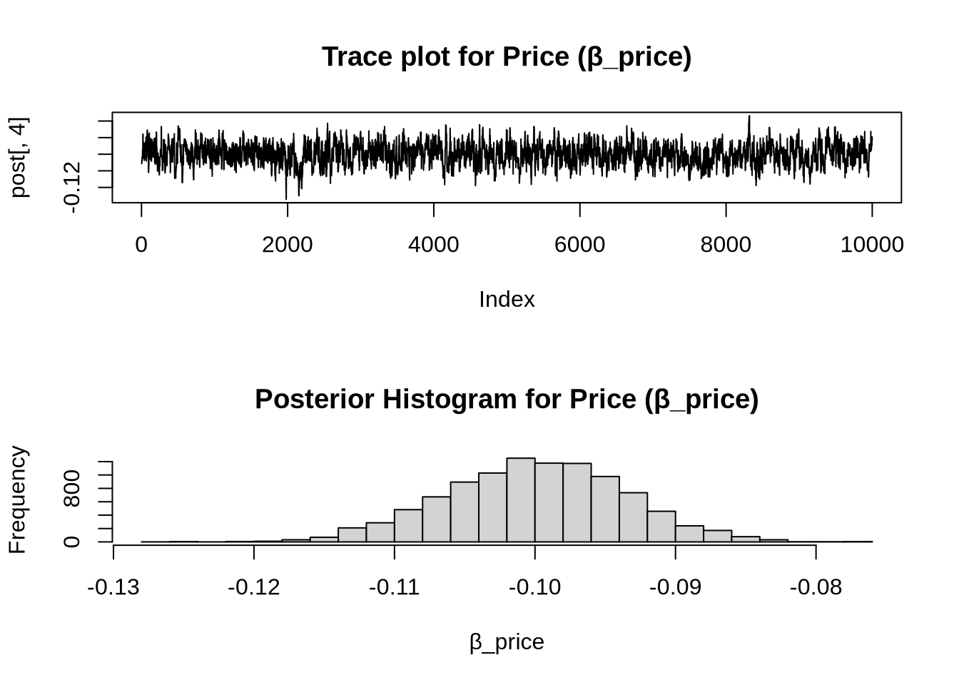

6. Discussion

Interpretation of Estimates

• β_Netflix > β_Prime:
  This means that, all else equal, consumers prefer Netflix over Amazon Prime. Since Hulu was the reference category (β = 0), the ordering of preference is: Netflix > Prime > Hulu.

• β_price < 0:
  A negative price coefficient makes intuitive sense — as price increases, the utility of the product decreases, making it less likely to be chosen. This aligns with rational consumer behavior.

• These signs are consistent with what we’d expect even if the data weren’t simulated. The signs and magnitudes of the coefficients indicate realistic preferences and trade-offs.

Hierarchical (Multi-Level) Model Extension

To model real-world conjoint data, we typically use a hierarchical or random-parameters MNL model. In this model, we assume:

• Each individual has their own β vector (preferences),
• These individual-level βs are drawn from a population distribution, typically multivariate normal:
  β_i ∼ MVN(μ, Σ)

To simulate data: - Sample β_i for each individual from MVN(μ, Σ), - Then generate choices using those personalized β_i values.

To estimate such a model: - Use Bayesian techniques like Hierarchical Bayes (e.g., Gibbs sampling or MCMC), - Estimate both the individual-level β_i and the population-level parameters (μ and Σ).

This allows the model to account for heterogeneity in preferences, which is essential for more accurate demand prediction and targeting in real applications.