Blueprinty Case Study
Introduction
Blueprinty is a small firm that makes software for developing blueprints specifically for submitting patent applications to the US patent office. Their marketing team would like to make the claim that patent applicants using Blueprinty’s software are more successful in getting their patent applications approved. Ideal data to study such an effect might include the success rate of patent applications before using Blueprinty’s software and after using it. Unfortunately, such data is not available.
However, Blueprinty has collected data on 1,500 mature (non-startup) engineering firms. The data include each firm’s number of patents awarded over the last 5 years, regional location, age since incorporation, and whether or not the firm uses Blueprinty’s software. The marketing team would like to use this data to make the claim that firms using Blueprinty’s software are more successful in getting their patent applications approved.
Data
We begin by loading the dataset and performing exploratory analysis.
      patents     region   age  iscustomer
0           0    Midwest  32.5           0
1           3  Southwest  37.5           0
2           4  Northwest  27.0           1
3           3  Northeast  24.5           0
4           3  Southwest  37.0           0
...       ...        ...   ...         ...
1495        2  Northeast  18.5           1
1496        3  Southwest  22.5           0
1497        4  Southwest  17.0           0
1498        3      South  29.0           0
1499        1      South  39.0           0

[1500 rows x 4 columns]
| iscustomer |
|
|
|
|
| Non-Customer |
3.473013 |
3.0 |
2.225060 |
1019 |
| Customer |
4.133056 |
4.0 |
2.546846 |
481 |
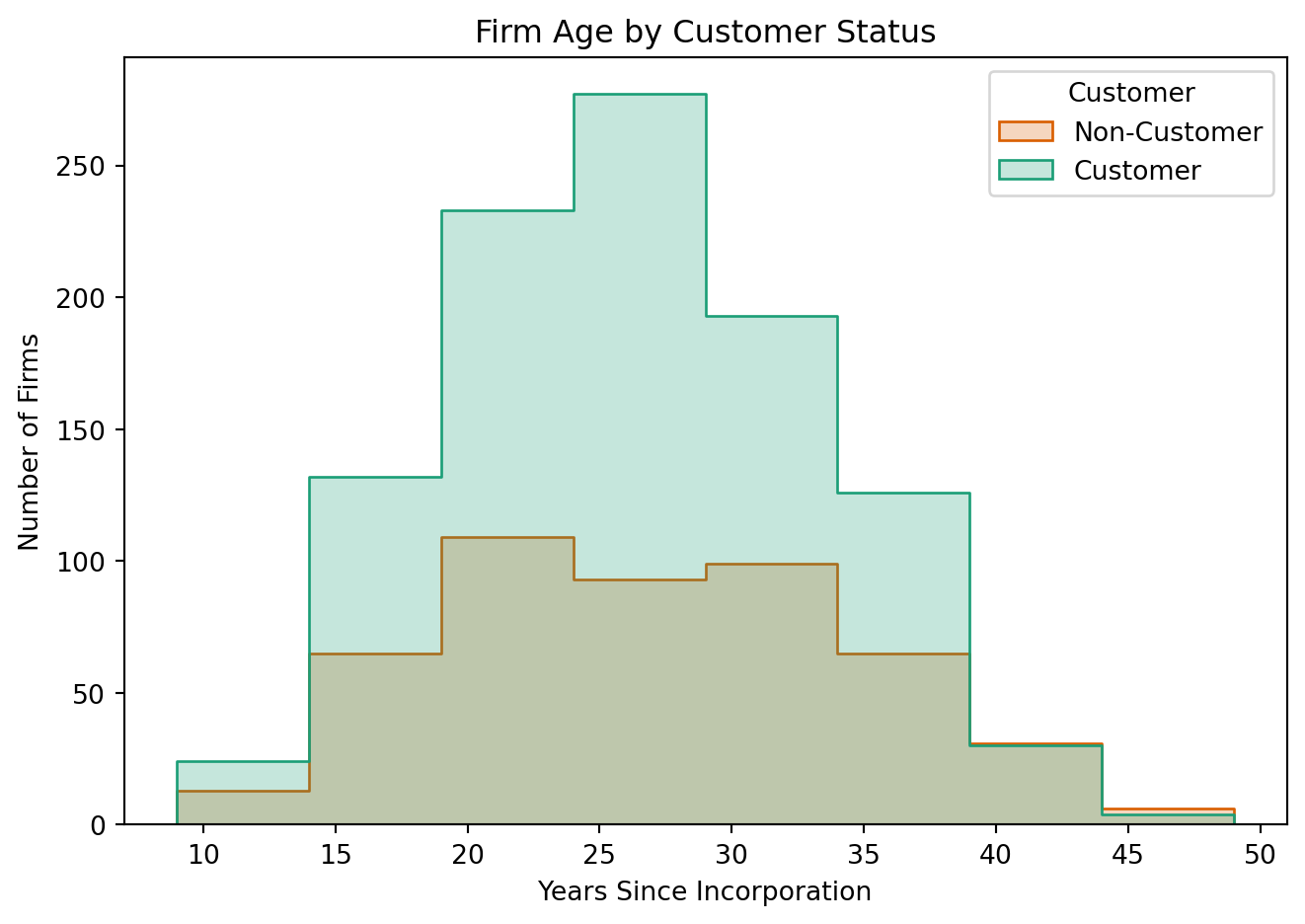
Next, we examine whether customer firms differ in age and regional location.
Blueprinty customers are not selected at random. It may be important to account for systematic differences in the age and regional location of customers vs non-customers.
| region |
|
|
| Midwest |
83.5% |
16.5% |
| Northeast |
45.4% |
54.6% |
| Northwest |
84.5% |
15.5% |
| South |
81.7% |
18.3% |
| Southwest |
82.5% |
17.5% |
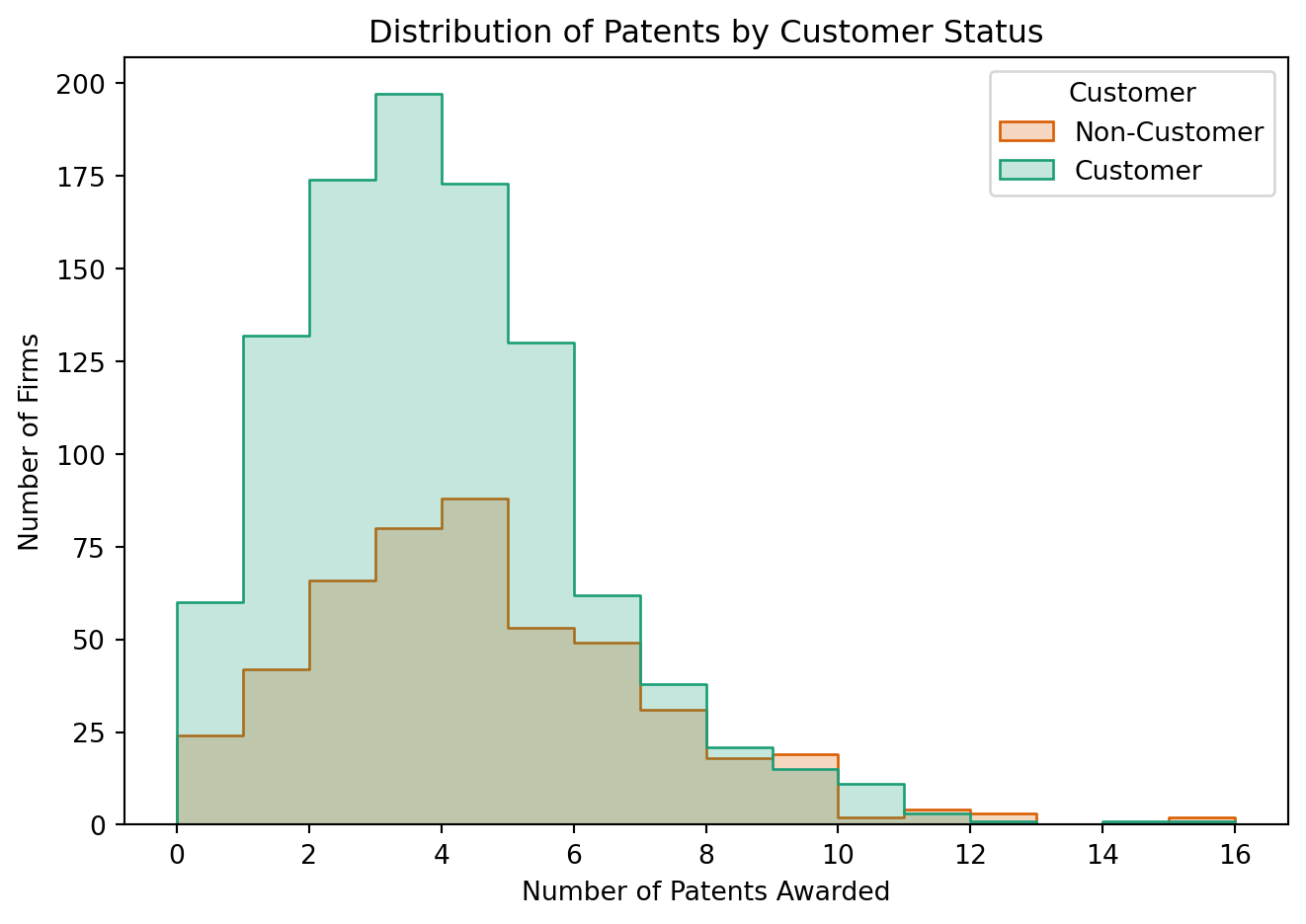
We observe that firms using Blueprinty tend to have more patents on average than those who do not. However, this raw difference may reflect underlying firm characteristics.
Estimation of Simple Poisson Model
Since our outcome variable of interest can only be small integer values per a set unit of time, we can use a Poisson density to model the number of patents awarded to each engineering firm over the last 5 years. We start by estimating a simple Poisson model via Maximum Likelihood.
Estimation of Simple Poisson Model
Since our outcome variable of interest can only be small integer values per a set unit of time, we can use a Poisson distribution to model the number of patents awarded to each engineering firm over the last 5 years. We start by estimating a simple Poisson model via Maximum Likelihood.
The probability mass function (pmf) of the Poisson distribution is:
\[
f(Y_i \mid \lambda) = \frac{e^{-\lambda} \lambda^{Y_i}}{Y_i!}
\]
Assuming independent observations across firms, the likelihood function for \(n\) firms is:
\[
\mathcal{L}(\lambda) = \prod_{i=1}^{n} \frac{e^{-\lambda} \lambda^{Y_i}}{Y_i!}
\]
Taking the log of the likelihood (to get the log-likelihood), we obtain:
\[
\log \mathcal{L}(\lambda) = \sum_{i=1}^{n} \left( -\lambda + Y_i \log \lambda - \log Y_i! \right)
\]
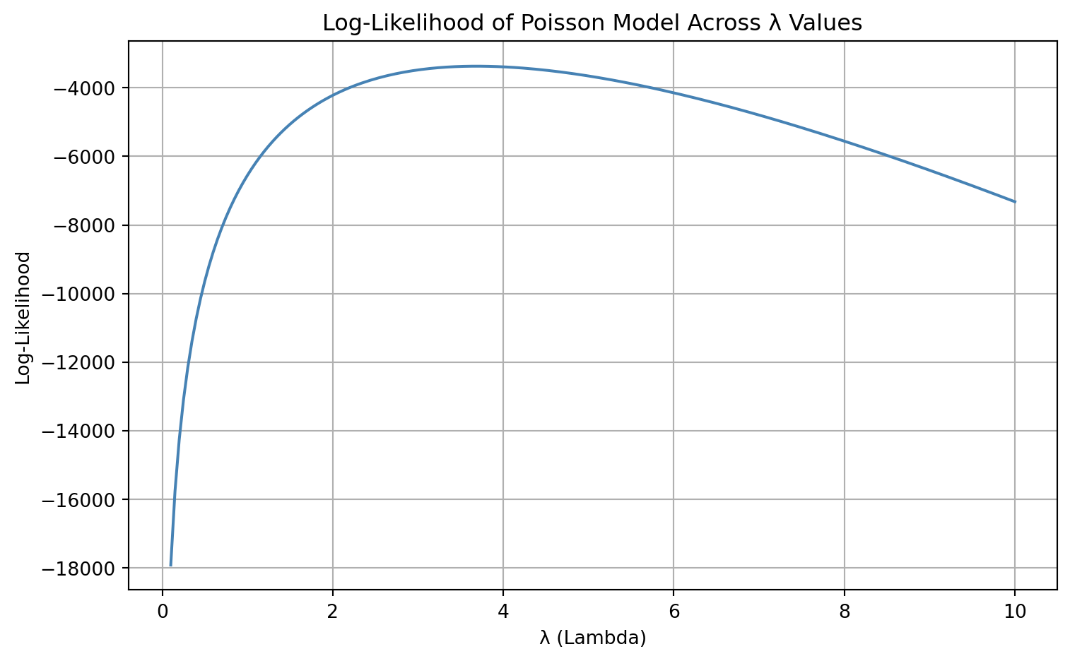
In the next step, we will numerically maximize this function to find the maximum likelihood estimate (MLE) of \(\lambda\).
poisson_loglikelihood <- function(lambda, Y){ … }
Analytical MLE Derivation
To find the MLE analytically, we take the derivative of the log-likelihood:
\[
\log \mathcal{L}(\lambda) = \sum_{i=1}^{n} \left( -\lambda + Y_i \log \lambda - \log Y_i! \right)
\]
Take the derivative with respect to \(\lambda\):
\[
\frac{d}{d\lambda} \log \mathcal{L}(\lambda) = \sum_{i=1}^{n} \left( -1 + \frac{Y_i}{\lambda} \right)
= -n + \frac{1}{\lambda} \sum_{i=1}^{n} Y_i
\]
Set this equal to 0:
\[
-n + \frac{1}{\lambda} \sum Y_i = 0 \quad \Rightarrow \quad \lambda_{\text{MLE}} = \frac{1}{n} \sum Y_i = \bar{Y}
\]
Thus, the maximum likelihood estimator of \(\lambda\) is simply the sample mean of the observed patent counts, which aligns with intuition: for a Poisson distribution, the mean and variance are both equal to \(\lambda\).
Estimation of Poisson Regression Model
Next, we extend our simple Poisson model to a Poisson Regression Model such that \(Y_i \sim \text{Poisson}(\lambda_i)\) where \(\lambda_i = \exp(X_i'\beta)\). The interpretation is that the rate of patent awards varies by firm characteristics \(X_i\).
We now update our log-likelihood function to be a function of a vector of regression coefficients \(\beta\) and a covariate matrix \(X\):
poisson_regression_likelihood <- function(beta, Y, X){
   ...
}
| Intercept |
1.480059 |
1.0 |
| C(region, Treatment)[T.Northeast] |
0.640979 |
1.0 |
| C(region, Treatment)[T.Northwest] |
0.164288 |
1.0 |
| C(region, Treatment)[T.South] |
0.181562 |
1.0 |
| C(region, Treatment)[T.Southwest] |
0.295497 |
1.0 |
| age |
38.016417 |
1.0 |
| age_sq |
1033.539585 |
1.0 |
| iscustomer |
0.553874 |
1.0 |
Generalized Linear Model Regression Results
| Dep. Variable: |
y |
No. Observations: |
1500 |
| Model: |
GLM |
Df Residuals: |
1492 |
| Model Family: |
Poisson |
Df Model: |
7 |
| Link Function: |
Log |
Scale: |
1.0000 |
| Method: |
IRLS |
Log-Likelihood: |
-3258.1 |
| Date: |
Mon, 09 Jun 2025 |
Deviance: |
2143.3 |
| Time: |
21:14:45 |
Pearson chi2: |
2.07e+03 |
| No. Iterations: |
5 |
Pseudo R-squ. (CS): |
0.1360 |
| Covariance Type: |
nonrobust |
|
|
|
coef |
std err |
z |
P>|z| |
[0.025 |
0.975] |
| Intercept |
-0.5089 |
0.183 |
-2.778 |
0.005 |
-0.868 |
-0.150 |
| C(region, Treatment)[T.Northeast] |
0.0292 |
0.044 |
0.669 |
0.504 |
-0.056 |
0.115 |
| C(region, Treatment)[T.Northwest] |
-0.0176 |
0.054 |
-0.327 |
0.744 |
-0.123 |
0.088 |
| C(region, Treatment)[T.South] |
0.0566 |
0.053 |
1.074 |
0.283 |
-0.047 |
0.160 |
| C(region, Treatment)[T.Southwest] |
0.0506 |
0.047 |
1.072 |
0.284 |
-0.042 |
0.143 |
| age |
0.1486 |
0.014 |
10.716 |
0.000 |
0.121 |
0.176 |
| age_sq |
-0.0030 |
0.000 |
-11.513 |
0.000 |
-0.003 |
-0.002 |
| iscustomer |
0.2076 |
0.031 |
6.719 |
0.000 |
0.147 |
0.268 |
Interpretation
The coefficient estimates from the Poisson regression using statsmodels.GLM() closely align with the MLE results we obtained using numerical optimization. This serves as a useful check and validates our earlier implementation.
Key interpretation points:
- Intercept: Represents the baseline log count of patents for a non-customer firm in the reference region (the region that was dropped in dummy encoding) with age and age² set to 0. While not directly interpretable on its own, it anchors the model.
- Age & Age Squared: The positive coefficient on
age and the (typically) negative coefficient on age_sq suggest a concave relationship: the number of patents increases with age, but at a decreasing rate.
- Customer Status (
iscustomer): A positive and statistically significant coefficient on this variable implies that, holding age and region constant, Blueprinty customers tend to have more patents than non-customers. This supports the marketing team’s hypothesis — but only after controlling for other variables.
- Region Dummies: These capture location-specific differences in patent productivity, relative to the omitted reference region.
Overall, the results suggest that firm age, region, and Blueprinty customer status are meaningful predictors of patent output.
Interpretation
To better understand the effect of Blueprinty’s software on patent success, we constructed two counterfactual scenarios:
X_0: all firms set as non-customers (iscustomer = 0)X_1: all firms set as customers (iscustomer = 1)
We used our fitted Poisson regression model to predict the number of patents for each firm under both scenarios. The difference in predicted patent counts reflects the causal effect of being a Blueprinty customer, holding all else constant.
We find that Blueprinty customers are predicted to receive, on average, 0.79 more patents over a 5-year period compared to non-customers with similar characteristics. This supports the marketing team’s claim that the software improves patent success, even after adjusting for firm age and region.